PostgreSQL Indexing Deep Dive: B-Tree, GIN, GiST, BRIN, and Index Maintenance
A step-by-step, practice-along guide to PostgreSQL indexing — from a no-index baseline through B-Tree, composite, partial, and covering indexes, Hash/GIN/GiST/BRIN, and production index maintenance, with runnable SQL and Python at every step.
Published on 16 jul 2026
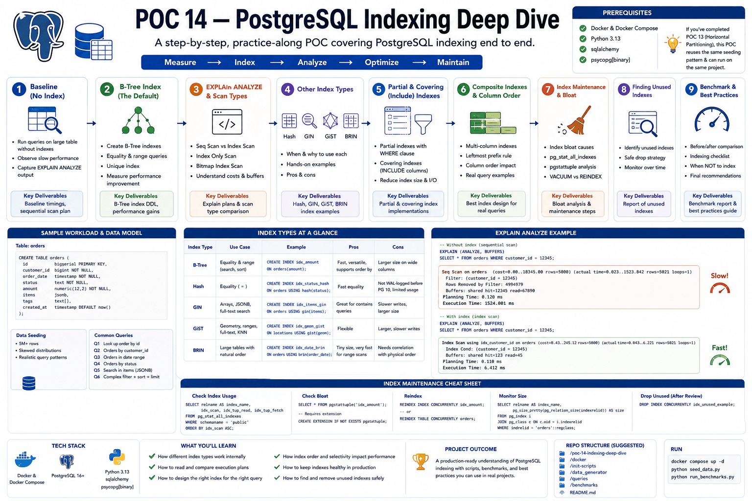
Table of Contents▶
- Goal
- Final Architecture
- Table of Contents
- Step 1 — Project Setup
- Step 2 — Baseline: Querying Without an Index
- Step 3 — Your First B-Tree Index
- Step 4 — Reading EXPLAIN ANALYZE: Scan Types
- Step 5 — Composite Indexes & Column Order
- Step 6 — Partial Indexes
- Step 7 — Covering Indexes (Index-Only Scans)
- Step 8 — Beyond B-Tree: Hash, GIN, GiST, BRIN
- Step 9 — Index Maintenance: Bloat, REINDEX, Unused Indexes
- Interview Questions Recap
- Completion Checklist
A step-by-step, practice-along POC covering PostgreSQL indexing end to end: baseline (no index) → B-Tree → EXPLAIN ANALYZE scan types → Hash/GIN/GiST/BRIN → partial & covering indexes → composite indexes & column order → index maintenance (bloat, REINDEX, finding unused indexes).
Prerequisites: Docker & Docker Compose, Python 3.13, sqlalchemy, psycopg[binary]. If you've completed POC 13 (Horizontal Partitioning), you already have the partition_demo database and seeding pattern this POC reuses — this POC can run standalone with its own database, or against that same project.
Goal
By the end of this POC you'll understand:
- Why sequential scans are slow, and how an index avoids them
- How a B-Tree index is structured internally
- How to read
EXPLAIN ANALYZEforSeq Scan,Index Scan,Index Only Scan, andBitmap Heap Scan - When to use Hash, GIN, GiST, and BRIN indexes instead of B-Tree
- Partial indexes and covering indexes
- Composite indexes and why column order matters
- Index bloat,
REINDEX, and finding unused indexes - Why indexing speeds up reads but costs on every write
Final Architecture
                    FastAPI
                        │
                        ▼
                  PostgreSQL
                        │
                     products
                        │
      ┌──────────┬──────────┬──────────┬──────────┐
      ▼          ▼          ▼          ▼
  B-Tree      GIN         GiST       BRIN
  (equality/  (full-text/ (geometry/ (huge, naturally
   range)      arrays/     ranges)    ordered data —
               jsonb)                 e.g. timestamps)
One table, several different indexes, each solving a different query shape.
Table of Contents
- Step 1 — Project Setup
- Step 2 — Baseline: Querying Without an Index
- Step 3 — Your First B-Tree Index
- Step 4 — Reading EXPLAIN ANALYZE: Scan Types
- Step 5 — Composite Indexes & Column Order
- Step 6 — Partial Indexes
- Step 7 — Covering Indexes (Index-Only Scans)
- Step 8 — Beyond B-Tree: Hash, GIN, GiST, BRIN
- Step 9 — Index Maintenance: Bloat, REINDEX, Unused Indexes
- Interview Questions Recap
- Completion Checklist
- What's Next
Step 1 — Project Setup
Folder Structure
indexing-poc/
│
├── docker-compose.yml
│
├── app/
│   ├── database.py
│   ├── seed.py
│   └── benchmark.py
│
├── sql/
│   └── schema.sql
│
├── requirements.txt
│
└── README.md
docker-compose.yml
version: '3.9'

services:
  postgres:
    image: postgres:17
    container_name: indexing-db
    restart: unless-stopped

    environment:
      POSTGRES_USER: postgres
      POSTGRES_PASSWORD: postgres
      POSTGRES_DB: indexing_demo

    ports:
      - '5433:5432'

    volumes:
      - indexing_data:/var/lib/postgresql/data

volumes:
  indexing_data:
Note: mapped to host port 5433 so it can run alongside the partition_demo container from POC 13 without a port clash.
Start PostgreSQL
docker compose up -d
docker ps
Expected container: indexing-db.
requirements.txt
fastapi
uvicorn[standard]
sqlalchemy
psycopg[binary]
app/database.py
from sqlalchemy import create_engine

DATABASE_URL = (
    "postgresql+psycopg://postgres:postgres@localhost:5433/indexing_demo"
)

engine = create_engine(
    DATABASE_URL,
    pool_pre_ping=True,
)
sql/schema.sql
A realistic products table we'll use for every index type in this POC:
DROP TABLE IF EXISTS products;

CREATE TABLE products (
    id BIGSERIAL PRIMARY KEY,
    sku VARCHAR(20) NOT NULL,
    name TEXT NOT NULL,
    description TEXT,
    category VARCHAR(50) NOT NULL,
    price NUMERIC(10,2) NOT NULL,
    status VARCHAR(20) NOT NULL DEFAULT 'ACTIVE',
    tags TEXT[],
    attributes JSONB,
    created_at TIMESTAMP DEFAULT CURRENT_TIMESTAMP
);
Notice this table intentionally has columns suited to different index types: sku/price (B-Tree), status (partial index candidate), tags (array → GIN), attributes (JSONB → GIN), created_at (naturally ordered, huge volume → BRIN candidate).
docker exec -i indexing-db psql \
-U postgres \
-d indexing_demo \
< sql/schema.sql
What You Learned
- Spinning up an isolated indexing sandbox alongside other POCs
- Designing one table that can demonstrate every index type covered in this POC
Step 2 — Baseline: Querying Without an Index
Rule: Never optimize before you have a baseline — same principle as the partitioning POC.
1. Seed the Table
app/seed.py
import random
import json

from sqlalchemy import text

from database import engine

TOTAL_ROWS = 500_000
BATCH_SIZE = 5000

categories = ["Electronics", "Clothing", "Home", "Toys", "Books", "Sports"]
statuses = ["ACTIVE", "ACTIVE", "ACTIVE", "DISCONTINUED", "OUT_OF_STOCK"]
all_tags = ["sale", "new", "clearance", "featured", "limited", "bestseller"]


def generate_batch(start_id):

    rows = []

    for i in range(BATCH_SIZE):

        product_id = start_id + i

        rows.append(
            {
                "sku": f"SKU-{product_id:08d}",
                "name": f"Product {product_id}",
                "description": f"Description for product {product_id}",
                "category": random.choice(categories),
                "price": round(random.uniform(5, 2000), 2),
                "status": random.choice(statuses),
                "tags": random.sample(all_tags, k=random.randint(1, 3)),
                "attributes": json.dumps(
                    {
                        "color": random.choice(["red", "blue", "green", "black"]),
                        "weight_kg": round(random.uniform(0.1, 20), 2),
                    }
                ),
            }
        )

    return rows


insert_sql = text(
    """
    INSERT INTO products
    (sku, name, description, category, price, status, tags, attributes)
    VALUES
    (:sku, :name, :description, :category, :price, :status, :tags, :attributes)
"""
)

with engine.begin() as conn:

    for start in range(0, TOTAL_ROWS, BATCH_SIZE):

        conn.execute(insert_sql, generate_batch(start))

        print(f"{start + BATCH_SIZE:,}/{TOTAL_ROWS:,}")

print("Done")
python app/seed.py
2. Run a Query With No Index
EXPLAIN ANALYZE
SELECT *
FROM products
WHERE sku = 'SKU-00250000';
Expected plan:
Seq Scan on products
  Filter: (sku = 'SKU-00250000'::text)
  Rows Removed by Filter: 499999
Planning Time: 0.1 ms
Execution Time: 45.xx ms
PostgreSQL had to check every one of the 500,000 rows to find the one matching row.
3. Benchmark It
app/benchmark.py
import time

from sqlalchemy import text

from database import engine

QUERY = text(
    """
    SELECT *
    FROM products
    WHERE sku = 'SKU-00250000'
"""
)

with engine.connect() as conn:

    start = time.perf_counter()

    rows = conn.execute(QUERY).fetchall()

    elapsed = time.perf_counter() - start

print(f"Rows : {len(rows)}")
print(f"Time : {elapsed:.4f} sec")
python app/benchmark.py
Save this number — this is your baseline.
What You Learned
- Why a
Seq Scanchecks every row - How to read
Rows Removed by Filteras a signal that an index would help - Establishing a measurable baseline before optimizing
Step 3 — Your First B-Tree Index
Why B-Tree?
B-Tree (Balanced Tree) is PostgreSQL's default index type, and the right choice for the large majority of cases: equality (=), ranges (<, >, BETWEEN), and sorting (ORDER BY).
B-Tree
↓
SKU-00250000
↓
Pointer
↓
Actual Row
1. Create the Index
CREATE INDEX idx_products_sku
ON products(sku);
2. Re-run the Query
EXPLAIN ANALYZE
SELECT *
FROM products
WHERE sku = 'SKU-00250000';
Expected plan now:
Index Scan using idx_products_sku on products
  Index Cond: (sku = 'SKU-00250000'::text)
Planning Time: 0.2 ms
Execution Time: 0.05 ms
3. Re-run the Benchmark
python app/benchmark.py
Compare against your Step 2 baseline — you should see a dramatic drop, often milliseconds instead of tens of milliseconds, and the gap widens as table size grows.
How a B-Tree Is Structured
                [ M ]
              /       \
         [ D, H ]     [ R, W ]
        /   |   \     /   |   \
      A-C  E-G  I-L  N-Q S-V  X-Z
Each level narrows the search range — lookups, range scans, and sorted output are all O(log n) instead of O(n).
The Cost: Slower Writes
EXPLAIN ANALYZE
INSERT INTO products (sku, name, category, price, status)
VALUES ('SKU-99999999', 'Test Product', 'Electronics', 99.99, 'ACTIVE');
Every insert now also has to insert into the B-Tree — cheap for one index, but the cost adds up with each additional index on the table.
What You Learned
- B-Tree is the default, general-purpose index
- How to read an
Index Scanplan - The
O(log n)structural reason B-Tree lookups are fast - Every index adds write overhead — there's no free lunch
Step 4 — Reading EXPLAIN ANALYZE: Scan Types
PostgreSQL's planner picks from several strategies. Recognizing each one in EXPLAIN ANALYZE output is a core production skill.
Seq Scan
Seq Scan on products
Reads every row, in physical order. Correct choice when there's no useful index, or when the query matches a large fraction of the table (an index would cost more than it saves).
Index Scan
Index Scan using idx_products_sku on products
  Index Cond: (sku = 'SKU-00250000'::text)
Walks the index to find matching entries, then fetches each matching row from the table ("heap") individually. Best when few rows match.
Bitmap Heap Scan / Bitmap Index Scan
EXPLAIN ANALYZE
SELECT *
FROM products
WHERE category = 'Electronics';
Bitmap Heap Scan on products
  Recheck Cond: (category = 'Electronics'::text)
  ->  Bitmap Index Scan on idx_products_category
        Index Cond: (category = 'Electronics'::text)
When many rows match (but not all), PostgreSQL builds an in-memory bitmap of matching row locations from the index, sorts it, then reads the table in physical order — fewer random-access reads than a plain Index Scan would need for that many matches.
Index Only Scan
Index Only Scan using idx_products_sku on products
  Index Cond: (sku = 'SKU-00250000'::text)
The fastest possible plan — the query is answered entirely from the index, without touching the table at all. Covered in depth in Step 7.
Comparison
| Scan Type | When PostgreSQL Chooses It |
|---|---|
| Seq Scan | No useful index, or query matches a large % of rows |
| Index Scan | Index exists, few rows match |
| Bitmap Heap Scan | Index exists, a moderate number of rows match |
| Index Only Scan | Index exists and covers every column the query needs |
What You Learned
- The four scan types you'll see constantly in production
EXPLAIN ANALYZEoutput - Why the planner sometimes chooses a Bitmap Heap Scan instead of a plain Index Scan
- That having an index doesn't guarantee it's used — the planner estimates cost and picks the cheapest plan
Step 5 — Composite Indexes & Column Order
The Problem
SELECT *
FROM products
WHERE category = 'Electronics'
AND status = 'ACTIVE'
ORDER BY price;
A single-column index on category alone still leaves PostgreSQL filtering status and sorting price the slow way after narrowing by category.
Creating a Composite Index
CREATE INDEX idx_products_category_status_price
ON products(category, status, price);
Why Column Order Matters
A composite B-Tree index is sorted left to right, like a phone book sorted by (last name, first name, city):
(Electronics, ACTIVE, 10.00)
(Electronics, ACTIVE, 15.00)
(Electronics, ACTIVE, 22.00)
(Electronics, DISCONTINUED, 8.00)
(Home, ACTIVE, 12.00)
...
This index is useful for:
WHERE category = 'Electronics'
WHERE category = 'Electronics' AND status = 'ACTIVE'
WHERE category = 'Electronics' AND status = 'ACTIVE' ORDER BY price
But it is not useful (on its own) for:
WHERE status = 'ACTIVE' -- skips the leading column, can't binary-search efficiently
Rule of thumb: put the column with equality filters first, then further equality filters, then the column used for ORDER BY or range comparisons last.
Verify with EXPLAIN ANALYZE
EXPLAIN ANALYZE
SELECT *
FROM products
WHERE category = 'Electronics'
AND status = 'ACTIVE'
ORDER BY price;
Expect an Index Scan (or Index Only Scan) using idx_products_category_status_price, with no separate sort step — the index already returns rows in price order for a fixed (category, status) pair.
What You Learned
- Composite indexes serve multi-column filters and sorts in one structure
- Column order determines which query shapes the index actually helps
- A composite index can also satisfy queries on its leading column(s) alone, but not on trailing columns in isolation
Step 6 — Partial Indexes
The Problem
SELECT *
FROM products
WHERE status = 'ACTIVE';
status has only a handful of distinct values (low cardinality). If 90% of rows are ACTIVE, a full index on status barely narrows anything down — and it still costs on every write, for every row, including the 10% you rarely query.
The Fix: Index Only the Rows You Actually Query
Suppose your application almost always searches for non-active products (to review discontinued or out-of-stock items) — a much smaller, more selective subset:
CREATE INDEX idx_products_inactive
ON products(sku)
WHERE status != 'ACTIVE';
Or, indexing only currently active products for a storefront that only ever lists active items:
CREATE INDEX idx_products_active_only
ON products(category, price)
WHERE status = 'ACTIVE';
Verify
EXPLAIN ANALYZE
SELECT *
FROM products
WHERE status = 'ACTIVE'
AND category = 'Electronics'
ORDER BY price;
The planner will use idx_products_active_only if the query's WHERE clause is a subset of the partial index's condition — PostgreSQL only allows this when it can prove the index's filter is satisfied.
Advantages
- Much smaller index → less memory, faster scans, faster writes for rows outside the partial condition
- Directly targets the actual access pattern instead of indexing everything "just in case"
The Catch
A partial index only helps queries whose WHERE clause matches (or is a stricter subset of) the partial index's condition. A query with a different or broader condition falls back to a full scan or a different index.
What You Learned
- Why low-cardinality columns are often poor candidates for a full index
- How a partial index targets exactly the subset of rows you query
- The condition-matching rule that determines whether the planner can use a partial index
Step 7 — Covering Indexes (Index-Only Scans)
The Problem
SELECT sku, price
FROM products
WHERE category = 'Electronics';
Even with an index on category, PostgreSQL still has to visit the actual table ("heap") to fetch sku and price for every matching row — an extra random-access read per row.
Index Scan
↓
Find matching rows in index
↓
Go to heap for sku, price   ← extra work
The Fix: INCLUDE Extra Columns
CREATE INDEX idx_products_category_covering
ON products(category)
INCLUDE (sku, price);
INCLUDE columns aren't part of the search key (they're not used for filtering or sorting), but they're stored right in the index — so once PostgreSQL finds a matching index entry, it already has everything the query asked for.
Verify
EXPLAIN ANALYZE
SELECT sku, price
FROM products
WHERE category = 'Electronics';
Expected:
Index Only Scan using idx_products_category_covering on products
  Index Cond: (category = 'Electronics'::text)
Heap Fetches: 0
Heap Fetches: 0 confirms the table itself was never touched — this is the fastest possible read plan.
Why Heap Fetches Isn't Always 0
Even with a covering index, PostgreSQL must still confirm row visibility (whether a row is visible to your transaction under MVCC) via the visibility map. If a page's visibility map bit isn't set (e.g. after heavy recent writes, before VACUUM has run), it still needs a heap fetch for those rows. Regular VACUUM keeps the visibility map up to date and Heap Fetches low.
Composite Search Key vs. INCLUDE Columns
-- Search key includes price (usable for filtering/sorting by price too)
CREATE INDEX idx_a ON products(category, price);

-- Search key is category only; price is just carried along
CREATE INDEX idx_b ON products(category) INCLUDE (price);
Use a full composite key when you filter or sort by the extra column; use INCLUDE when you only ever need to read that column's value once you've located the row, without filtering or sorting by it — this keeps the searchable part of the index smaller.
What You Learned
- What an Index Only Scan is and why it's the fastest possible plan
- How
INCLUDEbuilds a "covering" index without bloating the search key - Why
Heap Fetchescan be nonzero even with a covering index, and what keeps it low
Step 8 — Beyond B-Tree: Hash, GIN, GiST, BRIN
B-Tree isn't always the right tool. This step matches each remaining index type to the query shape it's built for.
Hash Index
Best for: pure equality (=) lookups only — no ranges, no sorting.
CREATE INDEX idx_products_sku_hash
ON products USING HASH (sku);
EXPLAIN ANALYZE
SELECT * FROM products WHERE sku = 'SKU-00250000';
In modern PostgreSQL, Hash indexes are WAL-logged and crash-safe, and can be marginally faster/smaller than B-Tree for pure equality — but they can't support <, >, BETWEEN, or ORDER BY at all. In practice, B-Tree is still the more common default even for equality-only cases, since it supports everything Hash does plus ranges and sorting; reach for Hash only when you've measured a concrete benefit.
GIN (Generalized Inverted Index)
Best for: columns containing multiple values per row — arrays, JSONB, full-text search.
CREATE INDEX idx_products_tags
ON products USING GIN (tags);

CREATE INDEX idx_products_attributes
ON products USING GIN (attributes);
EXPLAIN ANALYZE
SELECT * FROM products WHERE tags @> ARRAY['sale'];

EXPLAIN ANALYZE
SELECT * FROM products WHERE attributes @> '{"color": "red"}';
GIN builds an index entry per element (per array item, per JSON key, per lexeme in full-text search) pointing back to the rows containing it — the inverse of a normal index, hence "inverted index."
GiST (Generalized Search Tree)
Best for: data with overlapping or spatial relationships — ranges, geometric types, nearest-neighbor search — where "does A contain/overlap B" matters more than strict equality/ordering.
CREATE EXTENSION IF NOT EXISTS btree_gist;

ALTER TABLE products ADD COLUMN price_range NUMRANGE;
UPDATE products SET price_range = numrange(price - 5, price + 5);

CREATE INDEX idx_products_price_range
ON products USING GIST (price_range);
EXPLAIN ANALYZE
SELECT * FROM products
WHERE price_range @> 100.0::numeric;
GiST is also the standard index type behind PostGIS geometry columns (geometry && geometry, nearest-neighbor <-> queries).
BRIN (Block Range Index)
Best for: very large tables where the indexed column is naturally correlated with physical row order — classic example: created_at on an append-only, time-ordered table (which is exactly the situation Range Partitioning targets too — they pair well together).
CREATE INDEX idx_products_created_at_brin
ON products USING BRIN (created_at);
EXPLAIN ANALYZE
SELECT * FROM products
WHERE created_at BETWEEN '2026-01-01' AND '2026-02-01';
Instead of indexing every row, BRIN stores the min/max value per block range (e.g. per 128 pages). It's dramatically smaller than a B-Tree — often a tiny fraction of the size — at the cost of being much less precise: it can only rule out entire block ranges, not individual rows, so it degrades if the column isn't well-correlated with physical storage order.
Index Type Comparison
| Type | Best For | Supports Range/Sort | Typical Size |
|---|---|---|---|
| B-Tree | Equality, ranges, sorting — the default | ✅ | Medium |
| Hash | Pure equality only | ❌ | Medium/Small |
| GIN | Arrays, JSONB, full-text search | Partial (containment) | Large |
| GiST | Ranges, geometry, nearest-neighbor | Partial (overlap) | Medium |
| BRIN | Huge, naturally-ordered append-only data | Partial (block-level) | Tiny |
What You Learned
- Why B-Tree isn't a universal answer
- Which query shapes push you toward Hash, GIN, GiST, or BRIN
- Why BRIN trades precision for a dramatically smaller footprint, and why it pairs naturally with time-based range partitioning
Step 9 — Index Maintenance: Bloat, REINDEX, Unused Indexes
Indexes aren't "set and forget" — they need ongoing care in a production system.
1. Index Bloat
Frequent UPDATE/DELETE activity leaves dead entries inside a B-Tree that aren't immediately reclaimed, so the index grows larger than the live data it represents.
Check index size:
SELECT
    indexrelname,
    pg_size_pretty(pg_relation_size(indexrelid)) AS index_size
FROM pg_stat_user_indexes
WHERE relname = 'products'
ORDER BY pg_relation_size(indexrelid) DESC;
If an index's size seems disproportionate to the table's row count, bloat is a likely cause.
Fix bloat with REINDEX:
REINDEX INDEX CONCURRENTLY idx_products_sku;
CONCURRENTLY rebuilds the index without holding a long-lived lock that blocks writes — essential on a live production table (the non-concurrent REINDEX INDEX is faster but locks the table for its duration).
2. Finding Unused Indexes
Every index you don't need is pure write overhead with no read benefit. Find candidates for removal:
SELECT
    schemaname,
    relname AS table_name,
    indexrelname AS index_name,
    idx_scan AS times_used,
    pg_size_pretty(pg_relation_size(indexrelid)) AS index_size
FROM pg_stat_user_indexes
WHERE idx_scan = 0
ORDER BY pg_relation_size(indexrelid) DESC;
An index with idx_scan = 0 after a representative period of production traffic has never been used by the planner — it's a strong candidate to drop.
DROP INDEX CONCURRENTLY idx_products_sku_hash;
3. Checking for Wrong or Redundant Indexes
SELECT
    indexrelid::regclass AS index_name,
    indrelid::regclass AS table_name,
    indkey
FROM pg_index
WHERE indrelid = 'products'::regclass;
Look for indexes that are strict prefixes of other, wider composite indexes on the same table (e.g. an index on (category) alone when (category, status, price) already exists) — the narrower one is usually redundant, since the wider composite index can already serve category-only queries.
4. Autovacuum and Index Health
autovacuum keeps the visibility map current (which keeps Index Only Scans fast, per Step 7) and reclaims dead tuples over time. Check its activity:
SELECT
    relname,
    last_vacuum,
    last_autovacuum,
    n_dead_tup
FROM pg_stat_user_tables
WHERE relname = 'products';
A high n_dead_tup relative to total rows, with last_autovacuum far in the past, signals tuning is needed (more aggressive autovacuum thresholds for high-churn tables).
Production Best Practices
- Index for the query, not the column. Match composite index column order and partial index conditions to actual
EXPLAIN ANALYZE-verified query patterns, not guesses. - Every index has a write cost. Periodically audit and drop unused indexes.
- Use
CONCURRENTLYforCREATE INDEX,REINDEX, andDROP INDEXon live tables to avoid blocking writes. - Monitor bloat and vacuum health, not just query latency — degradation often creeps in silently over months.
- Pick the right index type for the data shape — don't force B-Tree onto arrays/JSONB (use GIN) or onto huge naturally-ordered append-only columns (consider BRIN).
What You Learned
- What index bloat is and how to detect and fix it with
REINDEX CONCURRENTLY - How to find and remove unused indexes with
pg_stat_user_indexes - How to spot redundant composite indexes
- Why
autovacuumhealth matters for index performance, not just table performance
Interview Questions Recap
Q1. Does adding an index always make queries faster?
No — for queries that match a large fraction of the table, the planner may correctly choose a Seq Scan over an index, since random-access index lookups for most of the table can be slower than one sequential read.
Q2. Why would PostgreSQL ignore an index that exists on the filtered column?
Common reasons: the query matches too large a fraction of rows (planner prefers Seq Scan), statistics are stale (run ANALYZE), the column is wrapped in a function without a matching expression index (WHERE LOWER(email) = ... needs an index on LOWER(email), not email), or the composite index's leading column isn't part of the query's filter.
Q3. What's the difference between an Index Scan and an Index Only Scan?
An Index Scan finds matching entries in the index, then fetches the actual row data from the table. An Index Only Scan answers the query entirely from the index (and the visibility map) without touching the table at all — only possible when the index (via its search key and/or INCLUDE columns) contains every column the query needs.
Q4. Why does every additional index slow down writes?
Because every INSERT/UPDATE/DELETE must also update every index on that table, in addition to the table itself — N indexes means N extra structures to maintain per write.
Q5. When would you choose BRIN over B-Tree?
When the table is very large, the column is naturally correlated with physical insertion order (e.g. an append-only created_at timestamp), and you need range queries — BRIN gives up per-row precision for a dramatically smaller index footprint that's cheap to maintain at huge scale.
Q6. Indexing vs. Partitioning vs. Sharding — how do they relate?
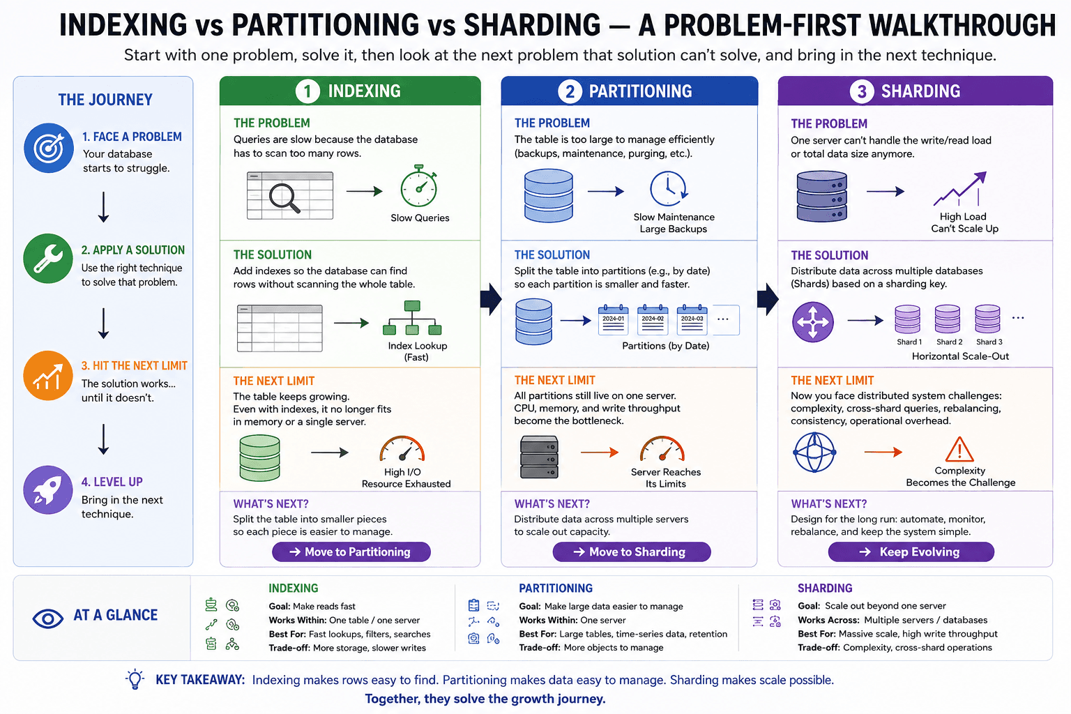
They solve different problems: indexing speeds up finding rows within a data set, partitioning reduces how much data must be considered within a single server by pruning irrelevant chunks, and sharding distributes data across multiple servers when a single server's hardware is the bottleneck. Production systems typically layer all three: shard across servers, partition each shard, and index within each partition.
Completion Checklist
- Project setup: Docker Compose,
database.py,productstable seeded with 500K rows - Baseline
Seq Scanbenchmark recorded (no index) - First B-Tree index created,
Index Scanverified, benchmark improvement measured - Read and distinguished Seq Scan / Index Scan / Bitmap Heap Scan / Index Only Scan
- Composite index created, column-order rule understood and verified
- Partial index created, condition-matching rule verified
- Covering index (
INCLUDE) created,Heap Fetches: 0confirmed - Hash index created and compared to B-Tree for equality-only lookups
- GIN index created for array/JSONB containment queries
- GiST index created for range/overlap queries
- BRIN index created for large, naturally-ordered time-series data
- Index bloat identified via
pg_stat_user_indexes, fixed withREINDEX CONCURRENTLY - Unused indexes identified via
idx_scan = 0and removed - Autovacuum / dead tuple health checked